Genotype quality control with plinkQC

Hannah Meyer and Maha Syed

2025-11-25

Introduction

Genotyping arrays enable the direct measurement of an individual’s genotype at thousands of markers. Subsequent analyses such as genome-wide association studies rely on the high quality of these marker genotypes.

plinkQC facilitates such genotype quality control, including a pre-trained ancestry classifier and relatedness filter optimized to retain the maximally unrelated sample set with highest quality.

plinkQC assumes the genotypes have already been determined from the original probe intensity data of the genotype array and are available in plink format. It wraps around PLINK [2] basic statistics (e.g. missing genotyping rates per individual, allele frequencies per genetic marker) and relationship functions. plinkQC then generates a per-individual and per-marker quality control report and individuals and markers that fail the quality control can subsequently be removed with plinkQC to generate a new, clean dataset.

The majority of functions in plinkQC depend on PLINK (version 1.9), which has to be manually installed prior to the usage of plinkQC. The ancestry functions depend on the newer version of PLINK 2.0 (version 2.0).

The protocol can be run via three main functions, the per-individual quality control (perIndividualQC), the per-marker quality control (perMarkerQC) and the generation of the new, quality control dataset (cleanData):

Per-individual quality control

The per-individual quality control with perIndividualQC wraps around these functions:

1. check_sex: for the identification of individuals with discordant sex information,

2. check_heterozygosity_and_missingness: for the identification of individuals with outlying missing genotype and/or heterozygosity rates,

3. check_relatedness: for the identification of related individuals

4. ancestry_prediction: for prediction of genomic ancestry

Per-marker quality control

The per-marker quality control with perMarkerQC wraps around these functions:

1. check_snp_missingnes: for the identifying markers with excessive missing genotype rates,

2. check_hwe: for the identifying markers showing a significant deviation from Hardy-Weinberg equilibrium (HWE),

3. check_maf: for the removal of markers with low minor allele frequency (MAF).

Clean data

cleanData takes the results of perMarkerQC and perIndividualQC and creates a new dataset with all individuals and markers that passed the quality control checks.

Workflow

In the following, genotype quality control with plinkQC is applied on a small example dataset with 200 individuals and 10,000 markers (provided within this package). The quality control is demonstrated in three easy steps, per-individual and per-marker quality control followed by the generation of the new dataset. In addition, the functionality of each of the functions underlying perMarkerQC and perIndividualQC is demonstrated at the end of this vignette.

To run the ancestry functionality of the package, Plink v2 is needed. Before use, the study data should be in the new hg38 annotation. USCS’s liftOver tool may be needed to map variants from one annotation to another. More details on how to use the tool can be found on the processing HapMap III reference data vignette. We provide an example dataset that is in the hg38 annotation.

Additional loading matrices are needed for the PCA projection used in the model. This is hosted on the plinkQC github repo under the inst/extdata folder located here. Alternatively, the whole github repo can downloaded with

git clone git@github.com:meyer-lab-cshl/plinkQC.git

The name of the files (before the .acount or .eigenvec.allele) for the loading matrices must be included in the path2load_mat variable.

package.dir <- find.package('plinkQC')
indir <- file.path(package.dir, 'extdata')
qcdir <- tempdir()
name <- 'data.hg38'
path2plink <- "/path/to/plink"
path2plink2 <- "/path/to/plink2"
path2load_mat <- "path/to/load_mat/merged_chrs.postQC.train.pca"

Per-individual quality control

For perIndividualQC, one simply specifies the directory where the data is stored (qcdir) and the prefix of the plink files (i.e. prefix.bim, prefix.bed, prefix.fam). Per default, all quality control checks will be conducted.

In addition to running each check, perIndividualQC writes a list of all fail individual IDs to the qcdir. These IDs will be removed in the computation of the perMarkerQC. If the list is not present, perMarkerQC will send a message about conducting the quality control on the entire dataset.

The ancestry portion of the package requires data in PLINK 2.0 format (i.e pgen, pvar, psam files), and the variant identifiers should be formatted similar to the following example: 1:12345[hg38]. perIndividualQC will run the functions convert_to_plink2() and rename_variant_identifiers() to convert the data into PLINK 2.0 format and rename the variant identifiers respectively.

NB: There are limitations on CRAN file sizes. To reduce the data size of the example data in plinkQC, data.genome has already been reduced to the individuals that are related. Thus the relatedness plots in C only counts for related individuals only. For ancestry identification, the example dataset is very small (10k genotypes) and contains markers and individuals failing qc controls to showcase the plinkQC’s functionality. In practice this means that the overlap in genotypes between the study and reference data is only 597 SNPs (roughly 0.2%) of the reference dataset. Thus, additional noise is expected and visible in the ancestry plot below.

perIndividualQC displays the results of the quality control steps in a multi-panel plot.

fail_individuals <- perIndividualQC(indir=indir, qcdir=qcdir, name=name,
                            path2plink=path2plink, 
                            path2load_mat = path2load_mat,
                            path2plink2=path2plink2, 
                            excludeAncestry = c("Africa"),
                            interactive=TRUE, verbose=TRUE)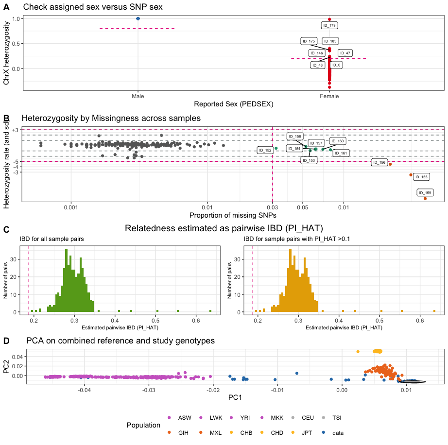

overviewperIndividualQC depicts overview plots of quality control failures and the intersection of quality control failures.

overview_individuals <- overviewPerIndividualQC(fail_individuals,
                                                interactive=TRUE)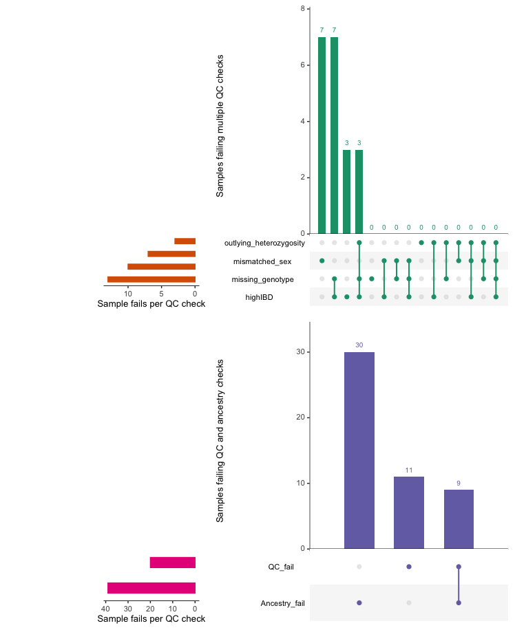

Per-marker quality control

perMarkerQC applies its checks to data in the specified directory (qcdir), starting with the specified prefix of the plink files (i.e. prefix.bim, prefix.bed, prefix.fam). Optionally, the user can specify different thresholds for the quality control checks and which check to conduct. Per default, all quality control checks will be conducted. perMarkerQC displays the results of the QC step in a multi-panel plot.

fail_markers <- perMarkerQC(indir=indir, qcdir=qcdir, name=name,
                            path2plink=path2plink,
                            verbose=TRUE, interactive=TRUE,
                            showPlinkOutput=FALSE)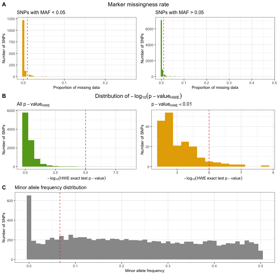

overviewPerMarkerQC depicts an overview of the marker quality control failures and their overlaps.

overview_marker <- overviewPerMarkerQC(fail_markers, interactive=TRUE)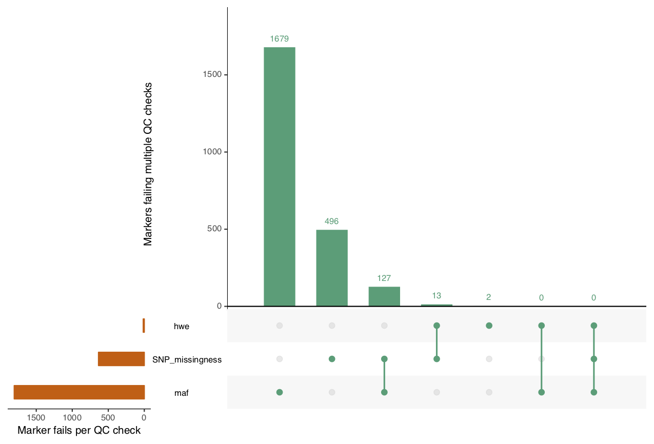

Create QC-ed dataset

After checking results of the per-individual and per-marker quality control, individuals and markers that fail the chosen criteria can automatically be removed from the dataset with cleanData, resulting in the new dataset qcdir/data.clean.bed,qcdir/data.clean.bim, qcdir/data.clean.fam. For convenience, cleanData returns a list of all individuals in the study split into keep and remove individuals.

Ids  <- cleanData(indir=indir, qcdir=qcdir, name=name, path2plink=path2plink,
                            verbose=TRUE, showPlinkOutput=FALSE)

Step-by-step

Individuals with discordant sex information

The identification of individuals with discordant sex information helps to detect sample mix-ups and samples with very poor genotyping rates. For each sample, the homozygosity rates across all X-chromosomal genetic markers are computed and compared with the expected rates (typically $<0.2$ for females and $>0.8$ for males). For samples where the assigned sex (PEDSEX in the .fam file) contradicts the sex inferred from the homozygosity rates (SNPSEX), it should be checked that the sex was correctly recorded (genotyping often occurs at different locations as phenotyping and misrecording might occur). Samples with discordant sex information that is not accounted for should be removed from the study. Identifying individuals with discordant sex information is implemented in check_sex. It finds individuals whose SNPSEX != PEDSEX. Optionally, an extra data.frame with sample IDs and sex can be provided to double check if external and PEDSEX data (often processed at different centers) match. If a mismatch between PEDSEX and SNPSEX was detected, by SNPSEX == Sex, PEDSEX of these individuals can optionally be updated. check_sex depicts the X-chromosomal heterozygosity (SNPSEX) of the samples split by their (PEDSEX).

fail_sex <- check_sex(indir=indir, qcdir=qcdir, name=name, interactive=TRUE,
                      verbose=TRUE, path2plink=path2plink)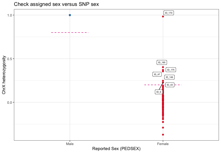

Individuals with outlying missing genotype and/or heterozygosity rates

The identification of individuals with outlying missing genotype and/or heterozygosity rates helps to detect samples with poor DNA quality and/or concentration that should be excluded from the study. Typically, individuals with more than 3-7% of their genotype calls missing are removed. Outlying heterozygosity rates are judged relative to the overall heterozygosity rates in the study, and individuals whose rates are more than a few standard deviations (sd) from the mean heterozygosity rate are removed. A typical quality control for outlying heterozygosity rates would remove individuals who are three sd away from the mean rate. Identifying related individuals with outlying missing genotype and/or heterozygosity rates is implemented in check_het_and_miss. It finds individuals that have genotyping and heterozygosity rates that fail the set thresholds and depicts the results as a scatter plot with the samples’ missingness rates on x-axis and their heterozygosity rates on the y-axis.

fail_het_imiss <- check_het_and_miss(indir=indir, qcdir=qcdir, name=name,
                                     interactive=TRUE, path2plink=path2plink)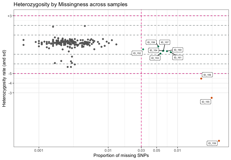

Related individualis

Depending on downstream analyses, it might be required to remove related individuals from the study. Related individuals can be identified by their proportion of shared alleles at the genotyped markers (identity by descend, IBD). Standardly, individuals with second-degree relatedness or higher will be excluded. Identifying related individuals is implemented in check_relatedness. It finds pairs of samples whose proportion of IBD is larger than the specified highIBDTh. Subsequently, for pairs of individual that do not have additional relatives in the dataset, the individual with the greater genotype missingness rate is selected and returned as the individual failing the relatedness check. For more complex family structures, the unrelated individuals per family are selected (e.g. in a parents-offspring trio, the offspring will be marked as fail, while the parents will be kept in the analysis).

NB: To reduce the data size of the example data in plinkQC, data.genome has already been reduced to the individuals that are related. Thus the relatedness plots in C only show counts for related individuals only.

exclude_relatedness <- check_relatedness(indir=indir, qcdir=qcdir, name=name,
                                         interactive=TRUE,
                                         path2plink=path2plink)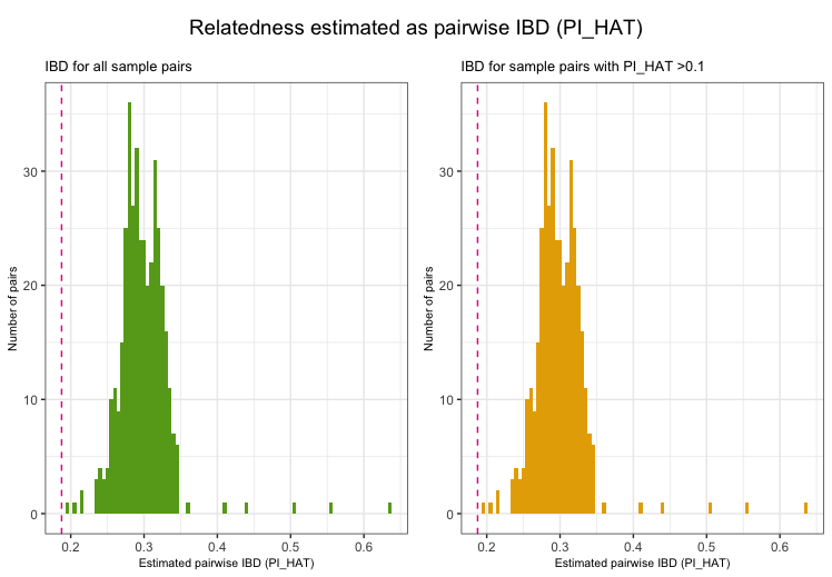

Ancestry Predictions of Data

For ancestry estimation, accessory functions from Plink v2 are needed, as are pre-computed loading matrices for the PCA projection used in the model. These are hosted on the plinkQC github repo under the inst/extdata folder located here. Alternatively, the whole github repo can downloaded with

git clone git@github.com:meyer-lab-cshl/plinkQC.git

For this, it is important that the data is in hg38 annotation. USCS’s liftOver tool may be needed to map variants from one annotation to another. More details on how to use the tool can be found on the processing HapMap III reference data vignette.

Additionally, the ancestry prediction function requires that the data is in plink 2 format and has variant identifiers in the format: 1:12345[hg38]. The function ancestry_prediction will call helper functions, convert_to_plink2() and rename_variant_identifiers() to format the data as directed by the parameters. The function returns: (i) prediction_prob: Dataframe of family ids, sample ids, and model probability of the each ancestry. (ii) prediction_majority: Dataframe of family ids, sample ids, and ancestry with highest model probability. (iii) exclude_ancestry: A list of ids to be excluded based on user-specified ancestries to the ancestral predictions of the samples (iv) p_ancestry: Bar graph of the ancestry model probabilities.

path2plink2 <- "/Users/syed/bin/plink2"
path2load_mat <- "path/to/load_mat/merged_chrs.postQC.train.pca"

anc_check <- ancestry_prediction(indir=indir, qcdir=qcdir, name=name,
                                         interactive=TRUE,
                                         path2plink2=path2plink2, 
                                         path2load_mat = path2load_mat)

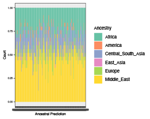
Markers with excessive missingness rate

Markers with excessive missingness rate are removed as they are considered unreliable. Typically, thresholds for marker exclusion based on missingness range from 1%-5%. Identifying markers with high missingness rates is implemented in snp_missingness. It calculates the rates of missing genotype calls and frequency for all variants in the individuals that passed the perIndividualQC.

fail_snpmissing <- check_snp_missingness(indir=indir, qcdir=qcdir, name=name,
                                         interactive=TRUE,
                                         path2plink=path2plink, 
                                         showPlinkOutput=FALSE)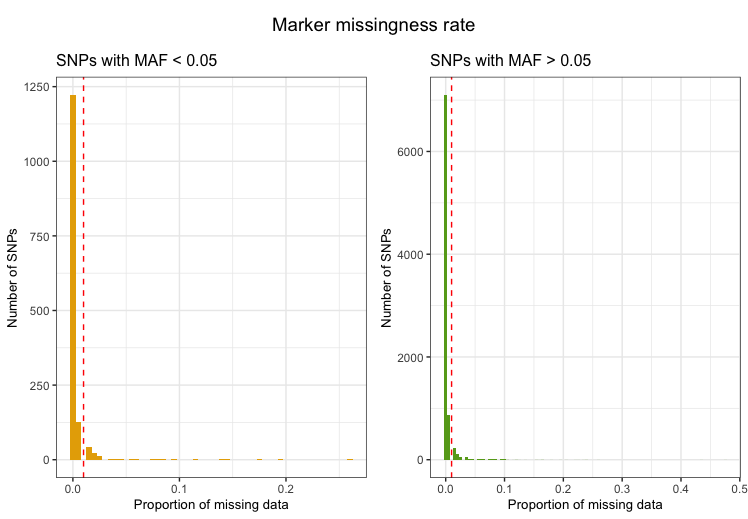

Markers with deviation from HWE

Markers with strong deviation from HWE might be indicative of genotyping or genotype-calling errors. As serious genotyping errors often yield very low p-values (in the order of $10^{-50}$), it is recommended to choose a reasonably low threshold to avoid filtering too many variants (that might have slight, non-critical deviations). Identifying markers with deviation from HWE is implemented in check_hwe. It calculates the observed and expected heterozygote frequencies per SNP in the individuals that passed the perIndividualQC and computes the deviation of the frequencies from Hardy-Weinberg equilibrium (HWE) by HWE exact test.

fail_hwe <- check_hwe(indir=indir, qcdir=qcdir, name=name, interactive=TRUE,
                      path2plink=path2plink, showPlinkOutput=FALSE)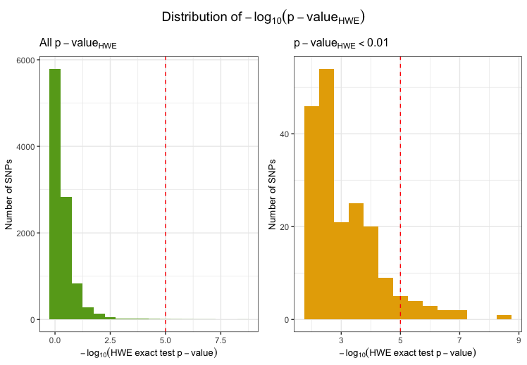

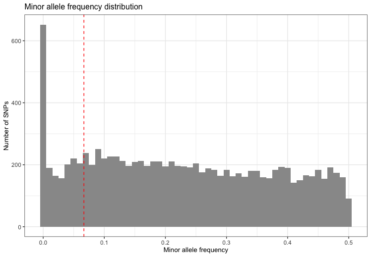
Markers with low minor allele frequency

Markers with low minor allele count are often removed as the actual genotype calling (via the calling algorithm) is very difficult due to the small sizes of the heterozygote and rare-homozygote clusters. Identifying markers with low minor allele count is implemented in check_maf. It calculates the minor allele frequencies for all variants in the individuals that passed the perIndividualQC.

fail_maf <- check_maf(indir=indir, qcdir=qcdir, name=name, interactive=TRUE,
                      path2plink=path2plink, showPlinkOutput=FALSE)

References

1.

Purcell S, Neale B, Todd-Brown K, Thomas L, Ferreira MAR, Bender D, et al. PLINK: a tool set for whole-genome association and population-based linkage analyses. The American Journal of Human Genetics. 2007;81: 559–75. doi:10.1086/519795

2.

Chang CC, Chow CC, Tellier LC, Vattikuti S, Purcell SM, Lee JJ. Second-generation PLINK: rising to the challenge of larger and richer datasets. GigaScience. 2015;4: 7. doi:10.1186/s13742-015-0047-8